Usage

denoise provides a command-line interface for training the Noise2Inverse model and denoising CT reconstructions.

Data preparation

Noise2Inverse requires two independent sub-reconstructions produced from complementary angular subsets of the raw projections (even-indexed and odd-indexed angles). These serve as training pairs: the network learns to predict one from the other, removing noise without any clean reference images.

Warning

A single full-angle reconstruction is not sufficient to run denoise. You must create the two sub-reconstructions from the raw projection data before proceeding.

Choosing a convolution mode

All denoise commands that touch the model accept a --mode flag:

`--mode`	Description	Typical use
`2.5d` (default)	2D U-Net; stacks N adjacent slices as channels. Fast and memory-efficient.	General synchrotron CT
`3d`	Full 3D U-Net with skip connections; operates on cubic sub-volumes. Removes structured 3D noise and ring artifacts.	Coherent X-ray / XNH microscopy

The mode is saved into the YAML config at the start of training, so you do not need to repeat --mode at inference time — the config already knows which model type was used. You can always override by passing --mode explicitly.

Note

The denoise slice command is only available in --mode 2.5d. In 3D mode, use denoise volume instead.

denoise prepare

Run denoise prepare (in the denoise environment) to write the config YAML and print the two tomocupy recon_steps commands you need to run next:

(denoise) $ denoise prepare --file-name /data/sample.h5

This reads instrument metadata from the HDF5 file, writes sample_rec_config.yaml, and prints the exact tomocupy recon_steps commands with the correct --out-path-name values.

Note

denoise prepare writes the config YAML only — it does not create the sub-reconstruction directories. Due to a NumPy compatibility issue between the denoise and tomocupy environments, the two sub-reconstructions must be created by running the printed commands manually in the tomocupy environment (see below). This limitation will be removed once the NumPy issue is resolved.

Sub-reconstructions with tomocupy

Run tomocupy recon_steps twice with the same parameters as the full reconstruction, adding --start-proj, --proj-step 2, and --out-path-name to select even and odd projections respectively. tomocupy writes output to <parent>_rec/ by convention, so the sub-reconstructions land next to the full reconstruction automatically:

# even-indexed projections (0, 2, 4, ...)
(tomocupy) $ tomocupy recon_steps \
                 --start-proj 0 --proj-step 2 \
                 --out-path-name /local/data/tomo_rec/sample_rec_0 \
                 [... same options as the full reconstruction ...]

# odd-indexed projections (1, 3, 5, ...)
(tomocupy) $ tomocupy recon_steps \
                 --start-proj 1 --proj-step 2 \
                 --out-path-name /local/data/tomo_rec/sample_rec_1 \
                 [... same options as the full reconstruction ...]

This produces:

/local/data/tomo_rec/
    sample_rec/    ← full reconstruction (already exists)
    sample_rec_0/  ← even-angle sub-reconstruction (N2I input A)
    sample_rec_1/  ← odd-angle sub-reconstruction  (N2I input B)

Note

Use exactly the same pre-processing options (ring removal, phase retrieval, normalisation, rotation axis) for both sub-reconstructions as for the full reconstruction.

Note

Non-tomocupy or non-APS HDF5 data

If your raw data is not in the standard APS HDF5 format, or you prefer a reconstruction tool other than tomocupy, you can create the two sub-reconstructions with any tool and write the config file by hand.

Using tomopy / dxchange (for arbitrary data formats):

import tomopy, dxchange

proj, flat, dark, theta = dxchange.read_aps_2bm('raw_data.h5')
proj = tomopy.normalize(proj, flat, dark)

rec0 = tomopy.recon(proj[0::2], theta[0::2], algorithm='gridrec')
rec1 = tomopy.recon(proj[1::2], theta[1::2], algorithm='gridrec')
rec_full = tomopy.recon(proj, theta, algorithm='gridrec')

dxchange.write_tiff_stack(rec0,    'sample_rec_0/recon')
dxchange.write_tiff_stack(rec1,    'sample_rec_1/recon')
dxchange.write_tiff_stack(rec_full,'sample_rec/recon')

In both cases, use the same pre-processing options (ring removal, phase retrieval, normalisation) for both sub-reconstructions as for the full reconstruction.

Because denoise prepare was not used, no config file was written automatically. Create one manually by copying the baseline template:

(denoise) $ cp /path/to/Noise2Inverse360/baseline_config.yaml \
           /path/to/sample_rec_config.yaml

and setting the four path fields to match your directories.

The metadata: block (used by the model registry for matching) will not be present in a manually created config. You can add it by hand or leave it empty — training will proceed normally either way.

Practical example (APS 2-BM, February 2026 Chawla dataset):

# even-indexed projections
(tomocupy) $ tomocupy recon_steps \
                --file-name /data3/2BM/2026-02/Chawla/As-cast-Mod2-100mm_115.h5 \
                --reconstruction-type full \
                --rotation-axis 1625 \
                --propagation-distance 100 \
                --energy 30 \
                --retrieve-phase-method paganin \
                --retrieve-phase-alpha 0.0005 \
                --pixel-size 0.69 \
                --fbp-filter ramp \
                --remove-stripe-method fw \
                --start-proj 0 --proj-step 2 \
                --out-path-name /data3/2BM/2026-02/Chawla_rec/As-cast-Mod2-100mm_115_rec_0

# odd-indexed projections
(tomocupy) $ tomocupy recon_steps \
                --file-name /data3/2BM/2026-02/Chawla/As-cast-Mod2-100mm_115.h5 \
                --reconstruction-type full \
                --rotation-axis 1625 \
                --propagation-distance 100 \
                --energy 30 \
                --retrieve-phase-method paganin \
                --retrieve-phase-alpha 0.0005 \
                --pixel-size 0.69 \
                --fbp-filter ramp \
                --remove-stripe-method fw \
                --start-proj 1 --proj-step 2 \
                --out-path-name /data3/2BM/2026-02/Chawla_rec/As-cast-Mod2-100mm_115_rec_1

This produces:

/data3/2BM/2026-02/Chawla_rec/
    As-cast-Mod2-100mm_115_rec/    ← full reconstruction (already exists)
    As-cast-Mod2-100mm_115_rec_0/  ← even-angle sub-reconstruction
    As-cast-Mod2-100mm_115_rec_1/  ← odd-angle sub-reconstruction

Training

denoise train

Train the Noise2Inverse model. denoise train automatically launches torchrun with the correct settings — no manual torchrun invocation is required.

Note

denoise train internally sets PYTHONNOUSERSITE=1 to prevent user-local packages in ~/.local/ from shadowing the conda environment.

Before launching training, denoise train automatically searches the local model registry for a model trained under the same instrument conditions and prompts you with the result.

Case 1 — a compatible model already exists:

# 2.5D (default)
(denoise) $ denoise train --config /data/sample_rec_config.yaml --gpus 0,1

# 3D mode
(denoise) $ denoise train --config /data/sample_rec_config.yaml --gpus 0,1 --mode 3d

Registry search found 1 matching model(s):
  [1] 2BM_pink_30keV_FLIROryx_22150530  (9/9 criteria match — 100%)
       beamline:            2-BM
       mode:                pink
       energy:              30.0 keV
       type:                GGG:Eu - ESRF
       serial_number:       22150530
       exposure_time:       0.035 s
       binning_x:           2
       binning_y:           2
       registry path:       /home/beams/TOMO/.denoise/registry/2BM_pink_30keV_FLIROryx_22150530
A compatible model may already exist. Copy the registry path above as --model-dir for slice/volume inference.

Train a new model anyway? [y/N]

Press Enter (or N) to cancel and reuse the existing model. Enter y to proceed with a new training run.

Case 2 — no compatible model found:

(denoise) $ denoise train --config /data/sample_rec_config.yaml --gpus 0,1

Registry search: no matching models found. Existing models:
  - 2BM_pink_30keV_FLIROryx_22150530

Proceed with new training? [Y/n]

Press Enter (or Y) to start training. Enter n to cancel and inspect the listed models manually. If the registry is empty the message reads Registry search: registry is empty.

To skip the registry search entirely, add --no-search:

(denoise) $ denoise train --config /data/sample_rec_config.yaml --gpus 0,1 --no-search

Running multiple training jobs on the same node

torchrun binds to port 29500 by default. If you launch a second training job on the same machine (e.g. two datasets on a 4-GPU node), the second job will fail with EADDRINUSE. Use --master-port to assign a different port to each job:

# job 1 — GPUs 0,1, default port
(denoise) $ denoise train --config /data/delta_config.yaml --gpus 0,1 --no-search

# job 2 — GPUs 2,3, different port
(denoise) $ denoise train --config /data/beta_config.yaml --gpus 2,3 --no-search --master-port 29501

--master-port only needs to be set for the second (and subsequent) jobs; the first job can always use the default.

Launch training with two GPUs:

(denoise) $ denoise train --config /data/sample_rec_config.yaml --gpus 0,1

For single-GPU training:

(denoise) $ denoise train --config /data/sample_rec_config.yaml --gpus 0

Any number of GPUs can be used — just list all the IDs. For example, on a 4-GPU machine:

(denoise) $ denoise train --config /data/sample_rec_config.yaml --gpus 0,1,2,3

denoise train counts the comma-separated IDs and sets --nproc_per_node accordingly. DDP splits the mini-batch across all GPUs, so doubling the number of GPUs roughly halves the time per epoch.

Tip

With more GPUs the effective per-GPU batch size is mbsz / n_gpus. On a 4-GPU machine consider increasing mbsz in the config (e.g. 64 or 128 instead of the default 32) to keep each GPU fully utilised:

train:
  mbsz: 128

Progress is logged to ~/logs/denoise_<timestamp>.log and printed to the console with colour-coded levels. Training output (checkpoints, loss curves) is saved to <directory_to_reconstructions>/TrainOutput/.

Three checkpoints are saved independently during training — each updated in-place whenever a new best is found:

File	Criterion	Recommended use
`best_val_model.pth`	Lowest validation L1 loss	Inference (best visual quality)
`best_lcl_model.pth`	Lowest LCL regularisation loss	Default (conservative)
`best_edge_model.pth`	Highest Laplacian edge score	Sharpness-focused comparison

Note

If training is interrupted (e.g. OOM or scheduler walltime), all three checkpoints reflect the best values seen up to that point and are fully usable for inference. For example, training killed at epoch 1710/2000 produced best_val_model.pth at epoch 1705 (val loss 0.053) and best_edge_model.pth at epoch 1650 — both suitable for inference.

What the model learns

The Noise2Inverse model learns the noise statistics of the imaging system, not anything about the sample itself. The model is fully sample-independent and can be reused across datasets as long as the acquisition conditions remain the same.

The network characterises:

Detector read noise and dark current
Shot noise at the specific photon flux (energy × exposure × beam current)
Scintillator glow and afterglow patterns
Ring artifact signatures from detector pixel non-uniformity
Any systematic noise from the lens and optic combination

What does not affect reusability:

Sample composition, density, or size
Rotation axis position
Number of projections (within reason)
Binning (as long as psz in the config matches the binned pixel size)

When to reuse vs. retrain

Condition	Reuse model?	Action
Same beamline, same detector, same energy, same exposure	Yes	Use registry model directly
Same setup, different sample	Yes	Use registry model directly
Same setup, different binning	Yes (if `psz` adjusted)	Update `psz` in config
Same setup, slightly different exposure (±20%)	Likely yes	Try inference; retrain if quality is poor
Different energy or significantly different flux	No	Retrain on new sub-reconstructions
Different detector or scintillator	No	Retrain on new sub-reconstructions
Different beamline	No	Retrain on new sub-reconstructions

Fine-tuning a pre-trained model

Instead of training from scratch, you can initialise the network with weights from a previously trained model and continue training on a new dataset. This is useful when acquisition conditions are similar but not identical — fine-tuning for a fraction of the original epochs may be sufficient:

# fine-tune from a registry entry
(denoise) $ denoise train \
                --config /data/new_sample_config.yaml \
                --gpus 0,1,2,3 \
                --finetune ~/.denoise/registry/2BM_pink_30keV_FLIROryx_22150530 \
                --no-search

# fine-tune from a specific .pth file
(denoise) $ denoise train \
                --config /data/new_sample_config.yaml \
                --gpus 0,1,2,3 \
                --finetune /data/brain_beta/TrainOutput/best_val_model.pth \
                --no-search

--finetune loads model weights only — all training state (epoch, loss history, best values) resets from scratch. When a registry directory is given, best_val_model.pth is used automatically.

Note

--finetune and --resume are mutually exclusive.

Resuming interrupted training

Every epoch, denoise train writes a resume.pth checkpoint to TrainOutput/ that captures the complete training state: model weights, optimiser state (Adam momentum), epoch counter, model_updates, all best values, and the full loss history. If training is interrupted for any reason, restart from the last completed epoch with --resume:

(denoise) $ denoise train --config /data/sample_rec_config.yaml --gpus 0,1 --resume

Training continues from epoch N+1 where N is the last fully completed epoch. All three best-model checkpoints are preserved and usable for inference at any point.

Note

resume.pth is overwritten at the end of every epoch. It is safe to run denoise slice or denoise volume while training is in progress — the inference commands load the best checkpoints, not resume.pth.

Warning

Do not use --resume after changing the config (e.g. psz, n_slices). You may safely increase maxep to extend training beyond the original limit.

Reducing training slices with z_stride

By default, all slices from the sub-reconstructions are loaded into RAM for training. For large CT datasets, adjacent slices are highly correlated along Z, so using every slice is rarely necessary. Set z_stride in the config to load only every Nth slice. This works in both 2.5D and 3D modes.

train:
  psz: 256
  n_slices: 5
  mbsz: 32
  lr: 0.001
  warmup: 2000
  maxep: 2000
  z_stride: 5   # use every 5th slice — 5× less RAM and 5× faster load

z_stride: 1 (the default) loads every slice. A value of 5 is a good starting point for brain-sized datasets (~2000 slices): it retains full anatomical coverage while reducing load time and memory by ~5×.

The warmup threshold is automatically divided by z_stride so that the number of warmup model updates stays proportional to the effective dataset size — no manual adjustment needed.

3D mode — RAM impact

In 3D mode each DDP rank loads the entire volume independently, so RAM scales as world_size × dataset_size. z_stride is especially important here. For a 1852-slice volume with two GPUs:

z_stride	Slices loaded	RAM per rank	Total (2 ranks)	Load time
1 (default)	1852	~430 GB	~860 GB	~14 min
5	370	~86 GB	~172 GB	~3 min
10	185	~43 GB	~86 GB	~90 s

The maximum useful z_stride is floor(D / psz_3d) — you must load at least psz_3d slices to draw a cubic training patch.

Note

Do not use --resume after changing z_stride in the config — the dataset size changes, which affects the epoch/update relationship.

Early stopping

By default, training runs for maxep epochs regardless of convergence. To stop automatically when the validation loss stops improving, add a patience key to the train section of the config:

train:
  psz: 256
  n_slices: 5
  mbsz: 32
  lr: 0.001
  warmup: 2000
  maxep: 2000
  patience: 200   # stop if val loss does not improve for 200 consecutive epochs

patience: 0 (the default) disables early stopping. The counter resets each time a new best validation loss is found and only starts after warmup completes. The state is saved in resume.pth so it is preserved across --resume restarts.

(denoise) $ denoise train -h
usage: denoise train [-h] --config FILE [--gpus IDS] [--mode MODE] [--resume] [--no-search] [--master-port PORT]

Train the Noise2Inverse model

options:
  -h, --help          show this help message and exit
  --config FILE       Path to the YAML configuration file
  --gpus IDS          Comma-separated list of visible GPU IDs (default: 0)
  --mode MODE         Convolution mode: 2.5d (default) or 3d
  --resume            Resume from the last completed epoch (requires resume.pth in TrainOutput/)
  --no-search         Skip registry search before training
  --master-port PORT  torchrun rendezvous port (default: 29500); change when running multiple jobs on the same node

3D mode configuration

When --mode 3d is passed to denoise train, the following YAML parameters control 3D training (denoise prepare always writes both 2.5D and 3D fields so no manual editing is required):

dataset:
  directory_to_reconstructions: /data/sample_rec
  sub_recon_name0: sample_rec_0
  sub_recon_name1: sample_rec_1
  full_recon_name: sample_rec

train:
  psz: 256          # 2.5D patch size (ignored in 3D mode)
  psz_3d: 96        # 3D cubic patch size — must be divisible by 2**n_blocks_3d
  n_slices: 5       # 2.5D stack depth (ignored in 3D mode)
  nb_patches_3d: 17600  # number of random 3D patches per epoch
  n_blocks_3d: 4    # U-Net encoder depth (matches SSD_3D reference)
  start_filts_3d: 56  # filter count of first encoder block
  mbsz: 4           # batch size — 3D patches are large; use 2–8 per GPU
  z_stride: 10      # load every 10th slice — critical for large volumes
  lr: 0.001
  warmup: 2000
  maxep: 2000
  patience: 0
  mode: '3d'        # saved automatically; read by slice/volume commands

infer:
  overlap: 0.5      # patch overlap fraction for 3D sliding window
  window: hann      # blending window (hann recommended for 3D)

Key differences from 2.5D config:

psz_3d replaces psz for 3D patch size. Must be divisible by 2**n_blocks_3d (e.g. 96 for 4 blocks since 96 / 16 = 6).
mbsz should be much smaller than in 2.5D — a 96³ patch at fp32 is ~3.4 MB, so 4–8 fit comfortably on a 40 GB GPU alongside the model.
nb_patches_3d sets how many random cubic patches are sampled per epoch. 17600 matches the SSD_3D reference; reduce for quick experiments or smaller volumes.
z_stride is especially important in 3D mode — each rank loads the full volume independently, so RAM scales as world_size × dataset_size. Use z_stride: 10 as a starting point for large volumes (>1000 slices).

Tip

The defaults written by denoise prepare (psz_3d: 96, n_blocks_3d: 4, start_filts_3d: 56, mbsz: 4) match the SSD_3D reference and are the recommended starting point. Reduce psz_3d to 64 (with n_blocks_3d: 3) if GPU memory is tight.

Inference

denoise slice (2.5D only)

Note

denoise slice is only available in 2.5D mode. In 3D mode, use denoise volume instead (single-slice inference is not meaningful for a model trained on cubic patches).

Tip

denoise slice can be run while training is still in progress. The model checkpoints in TrainOutput/ are updated in-place whenever a new best is found, so you can check denoising quality at any point without waiting for training to finish.

Denoise a single CT slice:

(denoise) $ denoise slice --config /data/sample_rec_config.yaml --slice-number 500
2025-01-01 10:00:00,000 - Loading slice 500
2025-01-01 10:00:05,000 - Saved denoised slice to .../sample_denoised_slices/00500.tiff

The denoised slice is saved as a TIFF in <directory_to_reconstructions>/<full_recon_name without _rec>_denoised_slices/.

By default the model is loaded from <directory_to_reconstructions>/TrainOutput/. To use a registered model instead, pass --model-dir:

(denoise) $ denoise slice \
                --config /data/sample_rec_config.yaml \
                --slice-number 500 \
                --checkpoint val \
                --model-dir ~/.denoise/registry/2BM_pink_30keV_FLIROryx_22150530_brain_beta_z5

(denoise) $ denoise slice -h
usage: denoise slice [-h] --config FILE [--gpus IDS] --slice-number N [--checkpoint {val,lcl,edge}] [--model-dir DIR]

Denoise a single CT slice

options:
  -h, --help                    show this help message and exit
  --config FILE                 Path to the YAML configuration file
  --gpus IDS                    Comma-separated list of visible GPU IDs (default: 0)
  --slice-number N              Index of the CT slice to denoise
  --checkpoint {val,lcl,edge}   Checkpoint to use (default: lcl)
  --model-dir DIR               Directory containing model checkpoints (default: TrainOutput/)

denoise volume

Note

The GPU batch size for inference is determined automatically by profiling the model against the configured patch size (psz) and the available GPU memory. On a modern GPU (e.g. A100 80 GB) the batch size will be maximised to saturate the GPU. For large volumes the initial RAM load (reading all TIFF files from disk) typically takes longer than the GPU inference itself.

Denoise the entire CT volume:

# 2.5D (default — or when mode is already stored in the config YAML)
(denoise) $ denoise volume --config /data/sample_rec_config.yaml

# 3D
(denoise) $ denoise volume --config /data/sample_rec_config.yaml --mode 3d
2025-01-01 10:00:00,000 - Loading data into CPU memory, it will take a while ...
2025-01-01 10:00:30,000 - Loaded 1000 slices of size 2048x2048
2025-01-01 10:00:30,100 - Patch volume size: 65536x256x256
2025-01-01 10:00:30,200 - Processing data ...
...
2025-01-01 10:05:00,000 - Stitching denoised data ...
2025-01-01 10:05:10,000 - Saving data to .../sample_denoised_volume ...
2025-01-01 10:05:30,000 - Done.

To denoise only a sub-volume (slices 200 to 400):

(denoise) $ denoise volume --config /data/sample_rec_config.yaml --start-slice 200 --end-slice 400

The denoised volume is saved as individual TIFF files in <directory_to_reconstructions>/<full_recon_name without _rec>_denoised_volume_<mode>/ (e.g. delta_all_denoised_volume_2.5d/ or delta_all_denoised_volume_3d/). This means results from both modes coexist in the same reconstruction directory without overwriting each other.

(denoise) $ denoise volume -h
usage: denoise volume [-h] --config FILE [--gpus IDS] [--start-slice N] [--end-slice N] [--checkpoint {val,lcl,edge}] [--model-dir DIR]

Denoise the entire CT volume

options:
  -h, --help                    show this help message and exit
  --config FILE                 Path to the YAML configuration file
  --gpus IDS                    Comma-separated list of visible GPU IDs (default: 0)
  --start-slice N               Start slice index (default: first slice)
  --end-slice N                 End slice index (default: last slice)
  --mode MODE                   Convolution mode: 2.5d (default) or 3d
  --checkpoint {val,lcl,edge}   Checkpoint to use (default: lcl)
  --model-dir DIR               Directory containing model checkpoints (default: TrainOutput/)

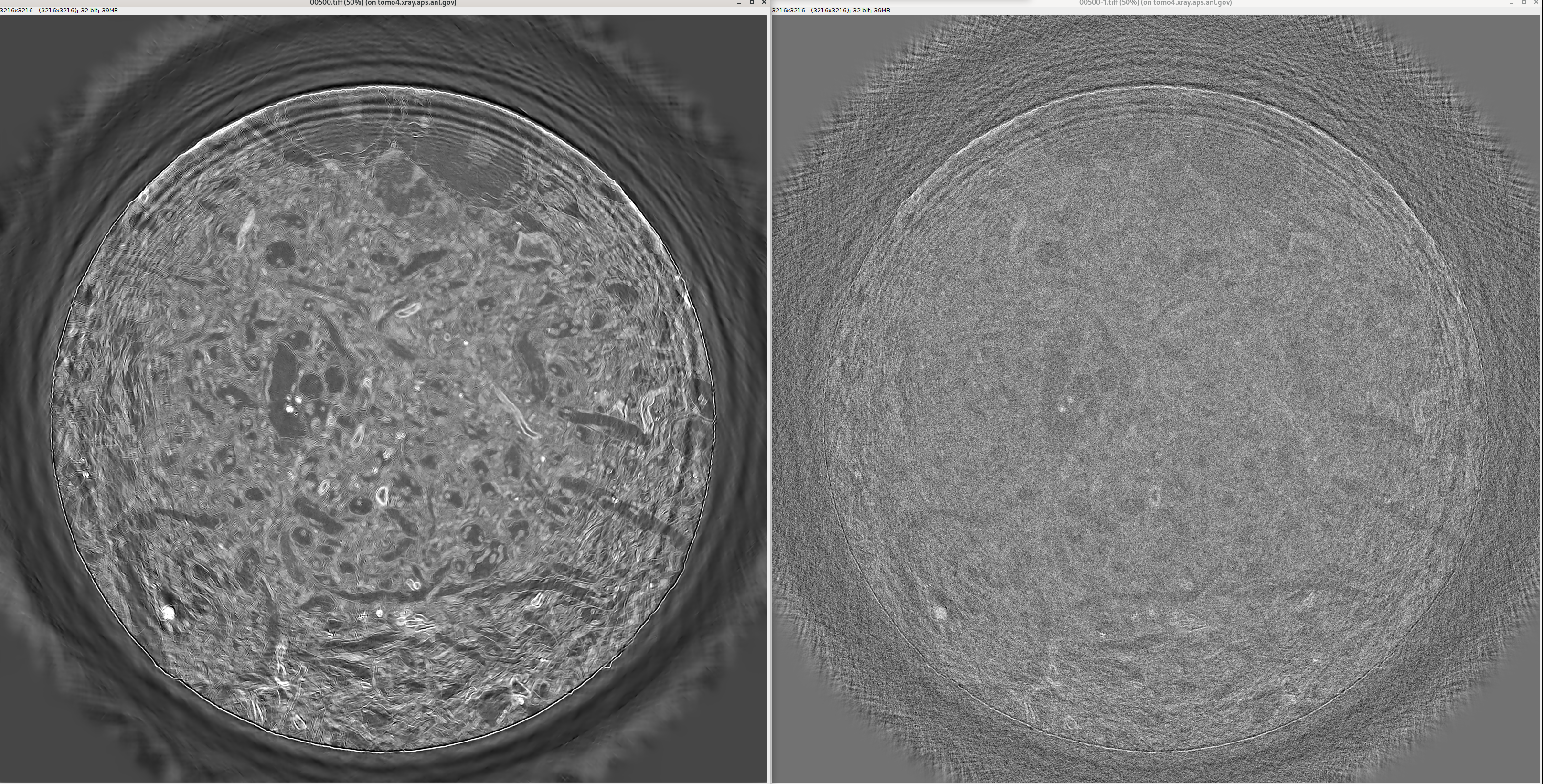
../_images/brain.png — Left: denoised — Right: noisy reconstruction (brain CT, APS 2-BM)

Performance example

The table below shows measured wall-clock times for a real APS 2-BM dataset:

Volume: 2426 slices × 3232 × 3232 voxels (~100 GB in RAM)
Training hardware: 2× NVIDIA V100 32 GB
Inference hardware: 1× NVIDIA A100 80 GB (batch size 512, auto-selected)

Two inference runs are shown — one with --checkpoint lcl (default) and one with --checkpoint val — to illustrate that checkpoint choice does not affect throughput: the model architecture is identical, only the weights differ.

Stage	`--checkpoint lcl`	`--checkpoint val`
Training (1710/2000 epochs, killed by SIGKILL at ~85%)	42 h 23 min	—
Load + normalize TIFFs into RAM	5 min 59 s	4 min 23 s
Pre-pad + build patch index	17 s	18 s
GPU inference (2962 batches × 512 patches)	41 min 45 s	41 min 13 s
Stitch patches → volume	11 min 16 s	16 min 58 s
Save 2426 TIFFs to disk	7 min 27 s	7 min 41 s
Total inference	~67 min	~71 min

GPU inference (~41 min, 60–62% of total) is stable across runs. Loading variation reflects OS disk-cache state. Stitching variation (~11–17 min) is due to system memory pressure. Training time dwarfs inference by ~38×; using 4 GPUs would reduce training to roughly 10–12 hours.

Model Registry

denoise includes a local model registry so that trained models can be stored, searched, and reused without manual bookkeeping. Models are stored in ~/.denoise/registry/ (override with the DENOISE_REGISTRY environment variable). Because tocai and tomo4 share the same home directory over GPFS, a model registered on tocai is immediately available on tomo4.

Note

The registry lives entirely in your home directory and is never tracked by git.

Instrument metadata in the config

When denoise prepare is run with --file-name, it reads key instrument parameters directly from the raw HDF5 file and writes them into the metadata: block of the generated config YAML:

metadata:
  start_date: '2026-02-19T09:02:27-0600'
  name: Chawla
  beamline: 2-BM
  current: 200.03 mA
  energy: 30.0 keV
  mode: pink
  type: GGG:Eu - ESRF
  active_thickness: 17.0 um
  magnification: 9.835
  resolution: 0.7015 um
  manufacturer: FLIR
  model: Oryx ORX-10G-310S9M
  serial_number: 22150530
  exposure_time: 0.035 s
  temperature: 25.3 C
  binning_x: 2
  binning_y: 2
  propagation_distance: 100.0 mm

This block is the basis for all registry matching. The fields used to decide whether two configs share the same noise fingerprint are:

beamline, mode, energy, type (scintillator), active_thickness, serial_number, exposure_time, binning_x, binning_y, and temperature (when present in both).

propagation_distance, magnification, current, and experimenter fields are recorded for provenance but are not used in matching.

Registering a trained model

After training is complete, register the model with its config:

(denoise) $ denoise register \
                --config /data/sample_rec_config.yaml \
                --model-dir /data/sample_rec/TrainOutput

An entry is created automatically under a name derived from the metadata (e.g. 2BM_pink_30keV_22150530_35ms_20260219_143000). To use a custom name:

(denoise) $ denoise register \
                --config /data/sample_rec_config.yaml \
                --model-dir /data/sample_rec/TrainOutput \
                --name 2BM_pink_30keV_FLIROryx

The registry entry contains a copy of the config and all three checkpoint files (best_val_model.pth, best_lcl_model.pth, best_edge_model.pth).

(denoise) $ denoise register -h
usage: denoise register [-h] --config FILE --model-dir DIR [--name NAME]

Register a trained model in the local registry for later reuse.

options:
  -h, --help        show this help message and exit
  --config FILE     Path to the YAML configuration file used for training
  --model-dir DIR   Directory containing the trained checkpoints (TrainOutput/)
  --name NAME       Registry entry name (auto-generated from metadata if omitted)

Searching the registry

To manually search the registry for models compatible with a given config:

(denoise) $ denoise search --config /data/new_sample_rec_config.yaml

Example output:

Registry search found 1 matching model(s):
  [1] 2BM_pink_30keV_FLIROryx_20260219_143000  (9/9 criteria match — 100%)
       beamline:            2-BM
       mode:                pink
       energy:              30.0 keV
       type:                GGG:Eu - ESRF
       serial_number:       22150530
       exposure_time:       0.035 s
       binning_x:           2
       binning_y:           2
       registry path:       /home/user/.denoise/registry/2BM_pink_30keV_FLIROryx_20260219_143000

(denoise) $ denoise search -h
usage: denoise search [-h] --config FILE

Search the registry for models trained under compatible instrument conditions.

options:
  -h, --help     show this help message and exit
  --config FILE  Path to the YAML configuration file to match against

Using a registered model for inference

When denoise train finds a matching model and you cancel training, create a new config for the new dataset (via denoise prepare) and add the normalisation statistics from the registered model’s config.yaml:

dataset:
  directory_to_reconstructions: /data/new_experiment
  sub_recon_name0: new_sample_rec_0
  sub_recon_name1: new_sample_rec_1
  full_recon_name: new_sample_rec
  mean4norm: 0.1234    # ← from the registered model's config.yaml
  std4norm:  0.0567    # ← from the registered model's config.yaml

Then run inference directly:

(denoise) $ denoise volume \
                --config /data/new_sample_rec_config.yaml \
                --checkpoint val

Note

mean4norm and std4norm are written by the training script and handle intensity normalisation. They must match the values used during training — copy them from the registered model’s config.yaml.

Command Reference

(denoise) $ denoise -h
usage: denoise [-h] ...

Noise2Inverse CT denoising library

options:
  -h, --help  show this help message and exit

Commands:

    prepare   Write a denoise config YAML from an HDF5 file path
    train     Train the Noise2Inverse model
    slice     Denoise a single CT slice
    volume    Denoise the entire CT volume
    register  Register a trained model in the local registry (~/.denoise/registry/)
    search    Search the registry for models matching a config noise fingerprint